India's Household Consumption Expenditure Survey (HCES) tracks household spending and provides data to assess living standards, estimate poverty and inequality, and inform national accounts.
From the early 1970s, the National Sample Survey (NSS) has been collecting household consumption data through large scale surveys carried out once in five years.[1] These quinquennial surveys have been used by both market research firms and policymakers to study consumption patterns across the country. India's official poverty figures were based on these surveys.[2]
Historically, these surveys were considered reliable enough to study poverty.[3] But since the 1980s, they have faced persistent criticisms for missing affluent households, and thereby underestimating the 'true' consumption levels in the country.[4] The growing gap between NSS estimates and the consumption expenditure estimates reported in India's national accounts statistics, or NAS,[5] added to such concerns.[6]
In this piece, we examine how affluent blocks have been sampled across NSS consumption surveys, how they differ from remaining blocks, and what changes in their coverage mean for interpreting recent trends in urban consumption.
How does the HCES sample affluent households?
In response to concerns over its surveys missing affluent households, the National Sample Survey Organisation (NSSO)[7] created distinct strata composed of affluent neighbourhoods[8] across major urban centres in the 1987-88 quinquennial round (43rd NSS round). A similar stratification strategy was also adopted in the next quinquennial round held in 1993-94 (50th NSS round).
Stratification involves dividing the population into population sub-groups in order to draw distinct samples from each of these sub-groups. The goal is to generate more reliable or precise estimates for each of the sub-groups and for the population as a whole.[9]
Each NSS survey typically has two levels of stratification. One kind of stratification is employed at the first stage of the sampling process to select a representative sample of household clusters (villages or urban blocks). After the 'first-stage' sampling units (FSUs) or clusters have been selected, another layer of stratification is used to select a desired sample of households or enterprises ('ultimate stage sampling units') from each of those clusters in the second stage of the sampling process. The first-stage stratification in NSS surveys is typically based on geographic markers (such as rural/urban) while the second-stage stratification is typically based on class-based markers (such as education or asset ownership).
For the first time in 1987-88, affluent neighbourhoods (blocks) were segregated in each major urban centre[10] at the first stage of the sampling process. The goal was to select adequate sampling units with high concentration of affluent households, raising the chances of capturing more affluent households in the urban sample.[11] After repeating the same stratification strategy in the 1993-94 round, NSSO dropped this strata in the subsequent quinquennial rounds.[12]
However, concerns about the growing NSS-NAS consumption gap led to a revival of the earlier stratification strategy in the 2022-23 and 2023-24 HCES rounds. An official committee set up to investigate the NSS-NAS gap in 2015 recommended a detailed study of the effect of the formation of "separate first-stage strata of affluent area blocks" to ensure "adequate representation of affluent households".[13]
How did the stratification strategy change in recent rounds?
Our analysis shows that the sample drawn from affluent blocks underwent significant changes in the 2022-23 and 2023-24 HCES rounds.
States from which affluent blocks were drawn
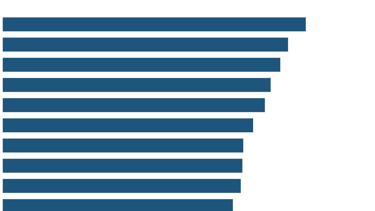
The first change relates to affluent strata being formed in a wider set of states in 2023-24. In 2022-23, affluent blocks were drawn from 12 of 36 states and union territories. Among 21 major states,[14] the exceptions were Andhra Pradesh, Assam, Bihar, Chhattisgarh, Jammu and Kashmir, Jharkhand, Kerala, Rajasthan, Telangana and Uttarakhand. In 2023-24, affluent blocks were drawn from 26 of 36 states and union territories. Among 21 major states, the only exceptions were Telangana and Uttarakhand.[15]
Size of urban centre
While affluent neighbourhoods were marked as separate strata only in the larger urban centres in the earlier rounds (1987-88, 1993-94), such strata were created even in smaller towns in the recent rounds.[16]
Across the four surveys, affluent blocks were selected from towns and cities of different sizes. In 1987-88 and 1993-94, affluent blocks were selected only in towns with at least 400,000 residents. The recent rounds, on the other hand, included affluent blocks across all town-size categories, including towns with fewer than 50,000 residents.
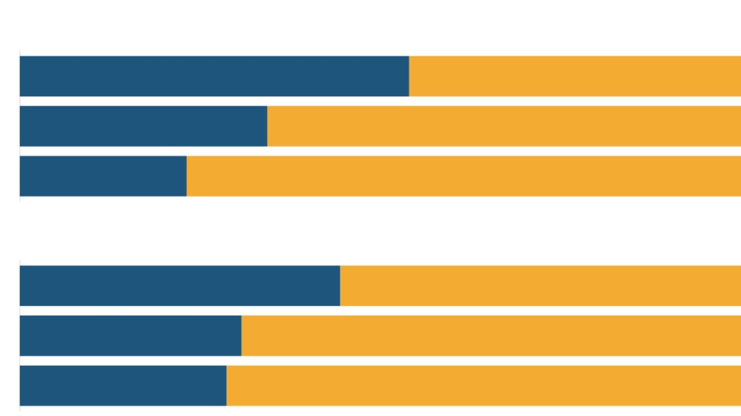
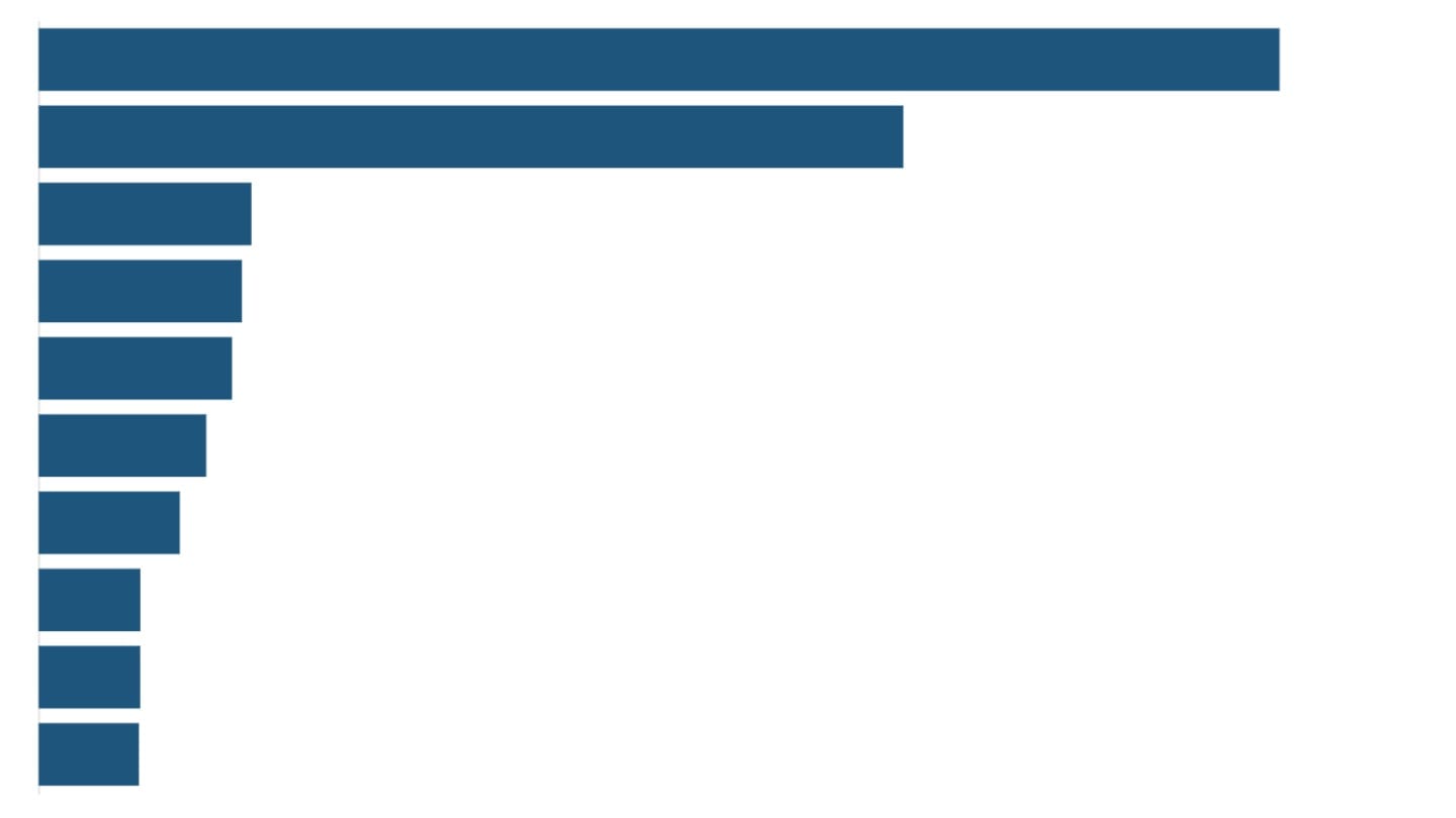
Moreover, the share of urban population represented by affluent blocks rose sharply between the two recent rounds, with the increase disproportionately concentrated in small and medium towns. Big cities[17] accounted for 32% of the population living in affluent strata in 2022-23, and only 18% in 2023-24. Correspondingly, the combined share of the population living in affluent blocks of small and medium towns[18] rose from 39% to 57%.
Share in urban households
Alongside this expansion in state coverage, affluent blocks' share of interviewed urban households increased only modestly, from 7.4% in 2022-23 to 8.5% in 2023-24. However, their weighted[19] share of all urban households rose sharply, from 1.1% to 7.5%. Their implied share of the urban population also increased, from about 1% to 7%. Consequently, their share of total urban consumption expenditure rose from 1.5% to 8.8% - roughly equal to Uttar Pradesh's share of India's urban consumption.
Does the current stratification capture the affluent?
Affluent blocks are indeed richer
In every round, the affluent strata's share in total consumption exceeded their share in the population, indicating higher average spending than in other urban blocks.
Households in affluent blocks were also more likely than those in non-affluent[20] blocks to be among urban India's highest spenders. In the recent two rounds, about 5% of households in affluent blocks belonged to the urban top 1% by monthly per capita consumption expenditure,[21] compared with about 1% of households in non-affluent blocks. Historical rounds too showed the similar pattern. In every round, households in affluent blocks were also more likely to belong to the urban top 5% and top 10%.
The affluent are different from the non-affluent socio-economically as well
The socio-economic characteristics of affluent blocks also appear to be markedly different from other neighbourhoods, in ways that correlate with affluence. Across all four surveys, affluent blocks had a higher proportion of residents with higher education and a smaller proportion of households dependent mainly on casual labour than non-affluent blocks. In 2023-24, 45% of residents aged 15 and above in affluent blocks had higher education, compared with 26% in non-affluent blocks. The gap was 52% versus 30% in big cities and 42% versus 22% elsewhere.
Affluent-block households were also less likely to depend mainly on casual labour: 6% versus 14% across urban India, 2% versus 8% in big cities, and 7% versus 16% in other cities and towns. Households in affluent blocks were twice as likely to have a laptop or computer (29% versus 15%) and nearly three times as likely to have a car (34% versus 12%). Across town types and survey rounds, affluent blocks showed similar differences in socio-demographic characteristics and asset ownership compared with non-affluent blocks. This suggests that affluent neighbourhoods have a distinct socio-economic composition compared with other neighbourhoods in the same cities.
Affluent blocks are not homogenous
At the first stage, the survey identifies each urban block as affluent or non-affluent; we refer to this as its area-level affluence status. At the second stage in the recent rounds, households within all selected blocks are grouped into three second-stage strata (SSS) based on car ownership. SSS-1 and SSS-2[22] comprise households that own at least one car, while SSS-3 comprises households that do not own a car.
In 2023-24, 34% of households in affluent blocks belonged to SSS-1 or SSS-2, the survey's car-owning household categories, compared with 12% in non-affluent blocks. The gap was similar in 2022-23: 32% versus 13%. This suggests that the affluent label helped identify areas with more such households. But how consistently did it do so across individual blocks?
To assess this, we checked whether individual blocks labelled affluent at the first stage also had a high concentration of relatively affluent households, using information recorded for second-stage stratification.
Regardless of area-level affluence status of a block, we classified it as 'affluent' if more than 25% of its households belonged to SSS-1 or SSS-2, and as 'non-affluent' otherwise. We refer to this as household-based affluence classifications. We then compared the area-level and household-based affluence classifications to see how often they agreed and where they differed.
In both recent rounds, only about half of the blocks marked affluent at the first stage qualified as affluent under this household-based criterion, while about one-sixth of blocks marked non-affluent also met the criterion. The correspondence was stronger in big cities, where roughly two-thirds of affluent-labelled blocks qualified, compared with about two-fifths in smaller cities and towns. The affluent-area label therefore captured a mixed set of neighbourhoods, with closer correspondence to household affluence in big cities.
Big city affluent blocks are distinct, and should be treated differently
The distribution of consumption expenditure across big city affluent neighbourhoods stands apart from the distribution in other urban blocks in the 1993-94, 2022-23, and 2023-24 consumption surveys. In big cities, affluent blocks had a higher concentration of the rich. In smaller urban centres, affluent blocks were relatively more heterogeneous.
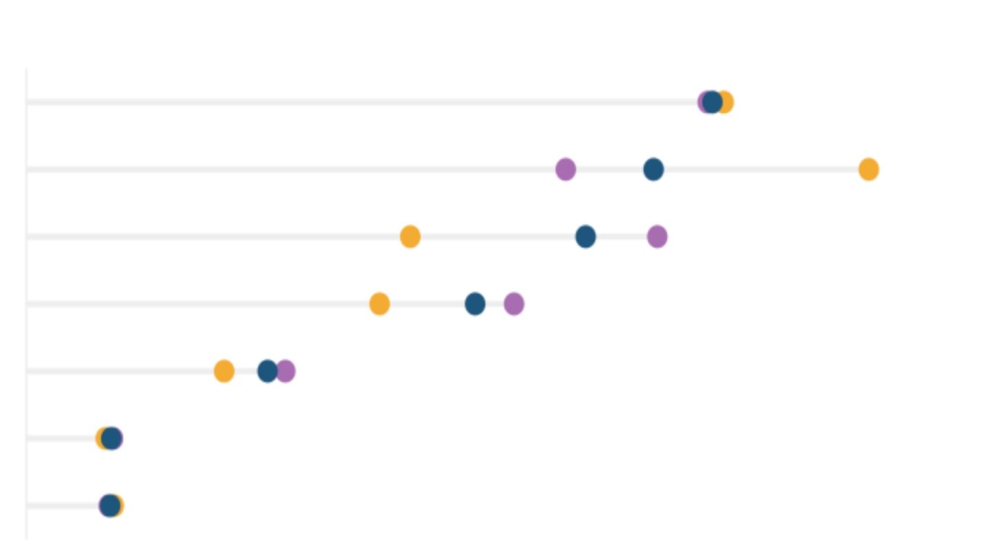
In the latest HCES round (2023-24), the monthly per capita consumption expenditure of affluent block households in big (million-plus) cities was 40% higher than that of non-affluent block households. In smaller cities and towns, the gap was relatively smaller: 32% in small towns, 25% in medium towns, and 21% in small cities.[23] The trends are broadly similar in the 2022-23 and 1993-94 consumption surveys as well. The differences between big city neighbourhoods and other urban blocks were relatively smaller in the 1987-88 round.
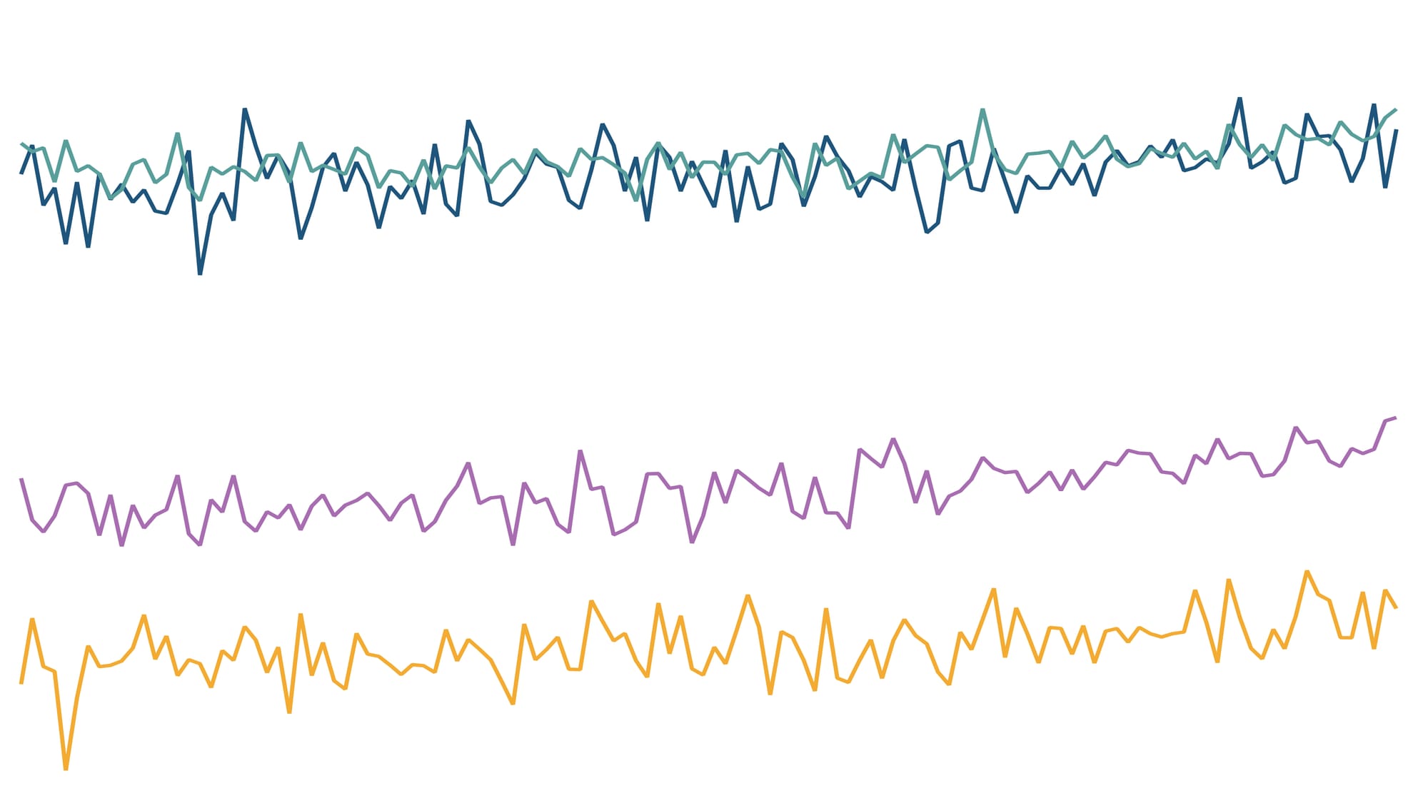
This matters because the data suggests that the per capita consumption of affluent blocks declined by 7% in 2023-24 compared to the previous year, even as per capita urban consumption grew 8.3% over the same period. The decline in affluent consumption was particularly sharp in Uttar Pradesh (-25%) and Gujarat (-12%).
The expanded coverage of affluent blocks in 2023-24 - with affluent blocks selected from a wider set of states - boosted the share of the affluent strata in overall urban consumption in the latest round. The greater weighted representation of affluent blocks in 2023-24 raised their share of total urban consumption expenditure from 1.5% to 8.8%. However, since the increase was lop-sided - with disproportionate increase in the smaller and poorer urban centres - it pulled down the average consumption levels of the affluent strata.
The changes between the two successive rounds could arise from changes made in the sampling frame,[24] random fluctuations in sampling, and intra-state changes in allocation of sampling units, the National Statistical Office (NSO) said in an emailed response to DFI's queries. States were considered as the 'basic stratum'[25] in both rounds, and hence sub-state results may not be consistent across the two rounds, NSO said. The question of why affluent blocks were selected from a smaller set of states in the 2022-23 survey (and from a much larger set of states in the next round) remained unanswered. Until these changes are better understood, year-on-year differences in affluent-block consumption cannot be read simply as changes in the living standards of a comparable population.
Non-response is a growing challenge
One challenge in sampling affluent households in recent rounds has been the growing rates of non-response among urban and richer households. The non-response rate is defined as the proportion of originally selected households in surveyed villages or blocks that were not interviewed, including those subsequently replaced by substitute households. Non-response may occur because household members are away, an informant is busy, the household does not cooperate, or for other reasons.
While rural non-response rates rose from 2.2% in 1993-94 to 5.4% in 2023-24, the urban non-response rate increased from 5.1% to 12.3% over the same time period. Within urban India, big cities tend to have higher levels of non-response compared to smaller urban centres. Within big cities, affluent blocks have much higher non-response rates compared to non-affluent blocks. The rates of substitution[26] have also gone up at a similar pace. This could pose challenges in accurately capturing the affluent.
Conclusion
Overall, the strategy of treating affluent neighbourhoods as a separate stratum seems to have worked in improving the representation of richer households in the HCES sample. However, affluent neighbourhoods in big cities are markedly different from those in urban centres. As a result, the changes within the affluent strata in the 2022-23 and 2023-24 rounds mean that the year-on-year changes in the consumption of affluent households may not reflect reality, and need to be interpreted with caution.
[1] Beginning with the first NSS round (1950-51), consumer expenditure data were collected in almost every round until 1973-74. Large-scale five-year (quinquennial) surveys began with the 27th round (1972-73). To provide consumption data between these surveys, smaller annual surveys, known as thin rounds, were introduced in 1986-87 and continued through 2007-08. See NSO's Household Surveys of NSS: A Journey of 75 Years.
[2] The last official poverty estimates were released in July 2013 by the Planning Commission. Based on consumer expenditure data from the NSS 68th round (2011-12) and poverty lines derived from the Tendulkar committee's recommendations, they placed 21.9% of India's population below the poverty line. No official consumption-based poverty headcount estimate has been released since then.
[3] The 55th round (1999-2000) is a big exception for comparisons over time. Drawing on a study by Professors T. J. Rao and A. K. Adhikary, the Tendulkar committee concluded that the published results of the 55th round cannot be made comparable with either the preceding 50th (1993-94) or the subsequent 61st (2004-05) round, mainly due to non-sampling errors introduced by using both 7-day and 30-day recall periods for certain food items in the same households in the 55th round. As Deaton and Kozel (2005) explain, "For high-frequency items, having both the 7-day and the 30-day reporting periods is likely to prompt respondents to reconcile the two reports."
[4] See Data and Dogma: The Great Indian Poverty Debate (2005), Deaton and Kozel, The World Bank Research Observer.
[5] The national accounts statistics (NAS) of a country provide a coherent set of estimates for major macro-economic parameters such as national income, overall consumption, investment, etc. The NSS-NAS consumption gap here refers to the difference between survey estimates of household consumption expenditure and NAS estimates of private final consumption expenditure (PFCE).
[6] According to the Adhikari committee's 2015 report, NSS estimates of household consumption were 5% below NAS estimates of private final consumption expenditure in 1972-73, 25% below in 1983-84, 50% below in 2004-05 and 45.2% below in 2011-12. Although the base years and survey recall periods differ across these estimates, the figures show that the gap widened substantially between 1972-73 and 2011-12.
[7] The National Sample Survey (NSS) began in 1950 as a programme of nationwide surveys. Initially, the Indian Statistical Institute (ISI) designed the surveys and prepared reports, while the Directorate of NSS conducted the fieldwork. These activities were brought together in the early 1970s under a new organisation, the National Sample Survey Organisation (NSSO), which became fully operational in 1972. In 2019, the NSSO was merged with the Central Statistical Organisation (CSO), established in 1951 to coordinate government statistics and later responsible for national income estimates, to form the National Statistical Office (NSO) and streamline statistical coordination and administration. See 75 Years of the Indian National Sample Survey (2025), G C Manna, Springer Nature.
[8] Affluent blocks are identified through the Urban Frame Survey (UFS). Field officials record up to two area types for each block, such as affluent, other residential, business/bazaar, slum or industrial. Affluent blocks contain a concentration of relatively affluent households within the town. To identify these blocks, the field officials apply their judgement or may take into account the views of their colleagues or other knowledgeable persons. Affluence is therefore a relative and partly subjective classification, which HCES uses alongside town size to form separate affluent and other-block strata.
[9] Stratification divides a population into groups and draws a separate sample from each. If the units (households or enterprises) within a group are relatively similar, its sample can give a more precise estimate of that group's average. Drawing samples separately also ensures that each group is represented. For example, a survey could sample affluent and other blocks separately, estimate average consumption in each, and combine those estimates according to the groups' shares of the population. This can improve the overall estimate when consumption differs between the groups. See Chapter 1 (pp. 49-50) of The Analysis of Household Surveys (1997), Angus Deaton, World Bank.
[10] Towns or cities with a population of 400,000 or more.
[11] See the Instructions to Field Staff, 43rd round (HCES 1987-88).
[12] In the 61st, 66th and 68th rounds, relatively affluent households within the selected first-stage units (FSUs) were placed in a separate sub-stratum, and comparatively larger samples were drawn from it instead of forming separate first-stage affluent strata. See Report of the Committee on Private Final Consumption Expenditure (2015), Adhikari et al., National Statistics Office.
[13] Report of the Committee on Private Final Consumption Expenditure (2015), Adhikari et al., National Statistics Office.
[14] States with a population of ten million or more as per the 2011 Census.
[15] In 1987-88, affluent blocks were selected from 13 of 30 states and union territories; among the 17 major states, the exceptions were Assam, Haryana, Odisha and Punjab. In 1993-94, affluent blocks were selected from 17 of 32 states and union territories; among the 17 major states, the exceptions were Assam, and Jammu and Kashmir.
[16] In both HCES 2022-23 and 2023-24, urban blocks within each state or union territory were classified by town size, based on the 2011 Census, and by their affluent-area status in the Urban Frame Survey. Towns with fewer than ten lakh population were grouped into three size classes: below 50,000; 50,000 to below three lakh; and three lakh to below ten lakh. Within each class, affluent blocks formed one stratum and the remaining blocks another. For towns with ten lakh or more population, each town had its own separate strata for affluent and remaining blocks.
[17] Cities with a population of one million or more, according to the 2011 Census
[18] Small towns refer to towns with fewer than 50,000 residents, and medium towns to those with 50,000 to fewer than 300,000 residents, according to the 2011 Census.
[19] Each household interviewed in a survey represents a certain number of households in the target population; this number is its survey weight, or multiplier, and can differ across households. An unweighted estimate counts each interviewed household equally and, in this case, shows the proportion of interviewed urban households drawn from affluent blocks. A weighted estimate counts each household according to its multiplier and, here, estimates the proportion of all urban households living in affluent blocks.
[20] This article uses "non-affluent blocks" for blocks that the survey did not mark as affluent and which the survey called "remaining" or "other" blocks.
[21] Monthly per capita consumption expenditure (MPCE) is calculated by dividing a household's monthly consumption expenditure by its number of members. For an area, total monthly consumption expenditure is divided by its total population. Consumption recorded over different recall periods is converted to a monthly equivalent.
[22] SSS-1 comprises households owning one or more cars for non-commercial use whose combined purchase price exceeded ₹10 lakh. SSS-2 comprises households owning such cars whose combined purchase price was ₹10 lakh or less.
[23] For the recent rounds, this article calls urban centres with fewer than 50,000 people "small towns"; those with 50,000 to below three lakh "medium towns"; those with three lakh to below ten lakh "small cities"; and those with ten lakh or more "big cities". The historical tables use a different grouping: towns below four lakh, small cities from four lakh to below ten lakh, and big cities with ten lakh or more.
[24] A sampling frame is the list of units from which a survey's sample is drawn. Urban HCES samples use blocks mapped through the Urban Frame Survey (UFS), which updates town maps and block characteristics, including affluent-area status, in five-year phases. So the latest available frame can contain blocks updated in different periods. The UFS data released in 2023 identify blocks from the 2007-12, 2012-17 and 2017-22 phases. As updates are spread across these phases, so available records can differ in "vintage"-the period when they were prepared or updated. According to MoSPI's methodological compendium, HCES 2022-23 used the 2012-17 UFS frame. For HCES 2023-24, the documentation mentions the latest available UFS frame without specifying its vintage. The precise difference in frame vintage between the two rounds is therefore unclear.
[25] A basic stratum is the smallest geographical unit for which a survey's sample is designed to support representative estimates. In HCES 2022-23 and 2023-24, states and union territories served as the basic stratum for forming strata and allocating the sample.
[26] Substitution rate is defined as the proportion of interviewed households that are substitutes. If an originally selected household cannot be surveyed in the first visit, an eligible household from the same second-stage stratum is selected in its place. If that substitute also cannot be surveyed, a second substitution is attempted. The HCES allow further attempts in exceptional cases to prevent a second-stage stratum from having no surveyed households.